Ordinary Least Squares: How to plot the line of best fit?

Ordinary least squares is a method to find parameters for a linear regression model. It helps to "fit" a function to a data by minimizing the sum of squared errors (residuals) from the data. Residual is the difference between the fitted line and the sample point.
But why minimize squared errors? Why not to minimize absolute errors? To understand this, lets look at the following example, from http://en.wikibooks.org/wiki/Econometric_Theory/Ordinary_Least_Squares_(OLS), where we plot sweater sales against temperature:

 http://en.wikibooks.org/wiki/Econometric_Theory/Ordinary_Least_Squares_(OLS)

 Notice that the sum of residuals in model A is 5+10-5-10 = 0 and sum of residuals in model B is 3-3+3-3 = 0. So are both models great fits?
No!
Clearly, it does not make rational sense to have a positive relation between sweater sales and temperature. Hence, we do not look to minimize errors but rather the squares of the errors in order to account for the sign.

Now how to fit a regression line to the above model? Say the model has an intercept β₀ and a slope term β_1. So we can write the model as:

y_i = β₀ + β₁x_i + u_i 

But it is not possible to find the values for β₀ and β₁, since these pertain to the population as a whole. So we take a sample from the population and estimate these values as shown in diagram below:

Chapter 2, Wooldridge, Jeffery M. 2006. Introductory Econometrics. 3td edition. Thomas South-western http://www.swlearning.com/economics/wooldridge/wooldridge2e/powerpoint.html

 

Now how to compute values for the sample parameters? The sum of squared residuals (SSR) is given by:

To minimize the SSR, we take the partial derivatives with respect to the sample parameters and equate to zero the two equations:

Now, simultaneously solving these equations, we get the following formulae for the sample parameters:

http://www.yongyoon.net/ecmetrics201/ols_derivation.pdf

For complete derivation of this result, view Derivation of OLS estimators

So this is basically how the method of least squares leads to a line of best fit!

Reference:

• Econometric Theory/Ordinary Least Squares (OLS)http://en.wikibooks.org/wiki/Econometric_Theory/Ordinary_Least_Squares_(OLS)
• Chapter 2, Wooldridge, Jeffery M. 2006. Introductory Econometrics. 3td edition. http://www.swlearning.com/economics/wooldridge/wooldridge2e/powerpoint.html
• Derivation of OLS estimators                                                    http://www.yongyoon.net/ecmetrics201/ols_derivation.pdf

How to achieve Pareto-optimal Allocation between two consumers?

First of all, what is a Pareto-optimal situation?

It is a situation in which no consumer can be made better off without making anyone else worse off. In economics, a situation that is not Pareto optimal implies that a certain reallocation of goods may result in some individual being made better off without making the other worse off. Hence, situations that are not Pareto optimal are to be avoided. (From Wikipedia, Pareto Efficiency)

But how to achieve Pareto-optimality?

To explain this, I make use of lecture slides from my Intermediate Microeconomics course at LUMS with Dr. Ali Hasanain. Lets assume that there are two consumers: A and B and their endowments of goods 1 and 2 are:

To show this in a diagram, I will use the Edgeworth box, which was devised by Edgeworth and Bowley to show all possible allocations of goods 1 and 2 between the two consumers. Lets see how to start with it:

Now, what allocations of 8 units of good 1 and 6 units of good 2 are feasible? How can all feasible allocations be depicted by the edgeworth box?
Basically, all points in the edgeworth box, including the boundary, represent feasible allocations between the two consumers. But which allocation can lead to a Pareto improvement i.e. which allocation can make both consumers better off?

To answer the question, we need to add preferences to the box. In economics, preferences are modelled by indifference curves which are set of all bundles of goods between which a consumer is indifferent i.e. these bundles are equally preferred by the consumer. For further elaboration on this concept, visit Indifference curve

Now, drawing the indifference curves for both A and B, we obtain:

All bundles above the indifference curves are more preferred. Now flipping the axes for B, and arranging both indifference curves together in the edgeworth box we obtain:

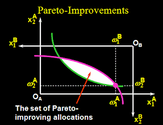
Now lets figure out the Pareto improving allocations. All points in the box, that lie above the indifference curves for both consumers represent Pareto improving situations, since they are preferred by both consumers simultaneously, as shown in the diagram below:

But which Pareto improving allocation will be the outcome of trade?

Now lets take a closer look at the indifference curves and find the situation that is Pareto optimal:

The above diagram shows the directions in which one consumer is better off and the other is worse off, as well as where both are worse off. Now coming back to our questions: which situation is Pareto optimal?

Here is the answer:

Therefore, an allocation where convex indifference curves are "only just back to back" is Pareto-optimal!                    

Reference:

• Pareto Efficiency, Wikipedia                                                                 http://en.wikipedia.org/wiki/Pareto_optimality
• Indifference Curve                                                                               http://en.wikipedia.org/wiki/Indifference_curve
• Lecture Slides by Dr. Ali Hasanain. Intermediate Microeconomics. Spring Semester 2010-2011.

 

What caused the Credit Crunch?

                                                           What is a Credit Crunch?

"A credit crunch (also known as a credit squeeze or credit crisis) is a reduction in the general availability of loans (or credit) or a sudden tightening of the conditions required to obtain a loan from the banks"   (http://en.wikipedia.org/wiki/Credit_crunch)

But what caused the Credit Crisis of 2008???

Several factors were responsible like:

- Sub-prime mortgages
                               - Collateralized debt obligations

                                                                          - Frozen credit markets

                                                                                                          - Credit default swaps

Don't know what these fancy terms mean?

For an illustrative explanation, view the following video:

http://www.youtube.com/watch?v=bx_LWm6_6tA&feature=related

Reference:

• Credit Crunch, Wikipedia                                                                                http://en.wikipedia.org/wiki/Credit_crunch
• The Crisis of Credit Visualized- HD                                                                                                 http://www.youtube.com/watch?v=bx_LWm6_6tA&feature=related

Prisoners' Dilemma: To confess or not to confess?

This post is about Game Theory, which is

"a mathematical method for analyzing calculated circumstances where a person's success is based upon the choices of others". (http://en.wikipedia.org/wiki/Game_theory)

For background on the game of prisoners' dilemma, please view the following video:

 http://www.youtube.com/watch?v=uX4CkBlXoxo

 Here is a matrix representation of this situation:

Bob\ Jack	Confess	Not confess
Confess	(3, 3)	(0.5, 5)
Not confess	(5, 0.5)	(1, 1)

The entries in the cells are the prison terms. For example, the entry that corresponds to (Confess, Not confess)- the entry in the first row second column- is the length of sentence to Bob (0.5) and Jack (5), respectively, when Bob confesses but Jack does not.
Now how do we determine the outcome of this game? What are the dominant strategies for each player?

Notice, if Jack plays "Confess", Bob will play "Confess" (since he prefers spending 3 years in prison rather than 5(if he does not confess)). Similarly, if Jack plays "Not confess", then Bob's best response is to "Confess". So, no matter what Jack plays, Bob's best reply is always "Confess". By the same logic, no matter what Bob plays, Jack's best reply is always "Confess" too.

     http://thebsreport.files.wordpress.com/2009/06/prisoner3.gif?w=875&h=580

Hence, (confess, confess) is a dominant strategy equilibrium in this game (Dutta, 1999).

However, this is not the most efficient outcome, since by not confessing, both players can simultaneously reduce their prison terms. But due to a lack of trust, the outcome (not confess, not confess) is not sustainable.

So next time, if you want two people to confess to their crime, you know what to offer them!!!

The game of prisoners dilemma has many real life applications especially in economics. A classic case is that of advertising where say two firms, A and B compete with each other. The profits each derive from advertising depends on the advertising conducted by the other firm. If both spend the same large amount in advertising, then their costs increase and no one benefits at the expense of the other. So both could reduce their costs (and increase their profits) by reducing advertising expenditure simultaneously. However, suppose if firm B decides not to spend on advertising, then firm A can benefit immensely by advertising. Since both firms cannot trust each other to advertise less, both end up advertising large equal amounts and making lesser profits.                                                       (http://en.wikipedia.org/wiki/Game_theory)

Reference:

• Game Theory                                                                                                                     http://en.wikipedia.org/wiki/Game_theory
• Dutta, Prajit K. (1999) Strategies and Games: Theory and Practice. The MIT Press: Cambridge, Massachusetts.
• Prisoner's Dilemma                                                                                                                            http://www.youtube.com/watch?v=uX4CkBlXoxo

How are Prices Determined in the Market?



http://www.glogster.com/media/4/24/17/18/24171889.jpg



Prices are determined by the forces of Demand and Supply.

The price which equates quantity demanded to quantity supplied is called equilibrium price. At this price, there is no tendency to change and buyers and sellers are both equally satisfied. At a price lower than the equilibrium price, quantity demanded exceeds quantity supplied, hence creating a shortage. Whereas, at a price above the equilibrium price, quantity supplied exceeds quantity demanded, hence creating a surplus. Therefore, any price below or above the equilibrium price is neither desirable nor sustainable, since there is a natural tendency to change (toward the equilibrium price). This is illustrated in the video below: 

http://www.youtube.com/watch?v=W5nHpAn6FvQ

Reference:

• Episode 14- Market Equilibrium                                                                                   http://www.youtube.com/watch?v=W5nHpAn6FvQ